
PSWS Ground Magnetometer Installation and Operation Manual
Raspberry-Pi RM3100 Magnetometer
The magnetic sensor for the PSWS project is an off-the-shelf, low-cost ($20) magnetic sensor using a new technology (“magneto-inductive”) with a noise floor of 4 pT/sqrt(Hz) at 1 Hz (PNI Geomagnetic Sensor RM3100, visit the website for more details). Regoli et al. (2018) demonstrated that the sensor performance is adequate for both space-borne and ground-based applications to study geomagnetic activity. Given that the sensor will be located in various electromagnetic environments, we expect the performance to be somewhat compromised and thus our target level is ~10 nT.
The RM3100 MI magnetometer consists of 1) single board computer (i.e. Raspberry Pi 3); 2) local magnetometer support board extender; and 3) remote magnetometer support board extender (see Figure 1). The remote board (Item #3) contains the RM3100 sensor which needs to be placed outside away from any sources of EMI while both the computer and local board are located inside. A recommended cable between the local and remote boards is a CAT5E or CAT6A shielded twisted pair (solid copper, NOT high resistance copper coated aluminum (CCA)).
The magnetometer package is expected to be in the range of $100 to $150. Again, the performance level of the magnetometer is lower (field resolution, in particular) than that of the high-performance, science-grade magnetometers deployed at geophysical observatories across the US. We note, however, that the proposed network is focused primarily on their spacing to increase the spatial resolution. Given the adequate resolution level (< 10 nT at 1 Hz), most of the major geomagnetic activity (e.g., geomagnetic storms, substorms (may be limited to high-latitude regions) and large-scale ULF waves/disturbances) is expected to be observed, which will be compared with the HF measurements.
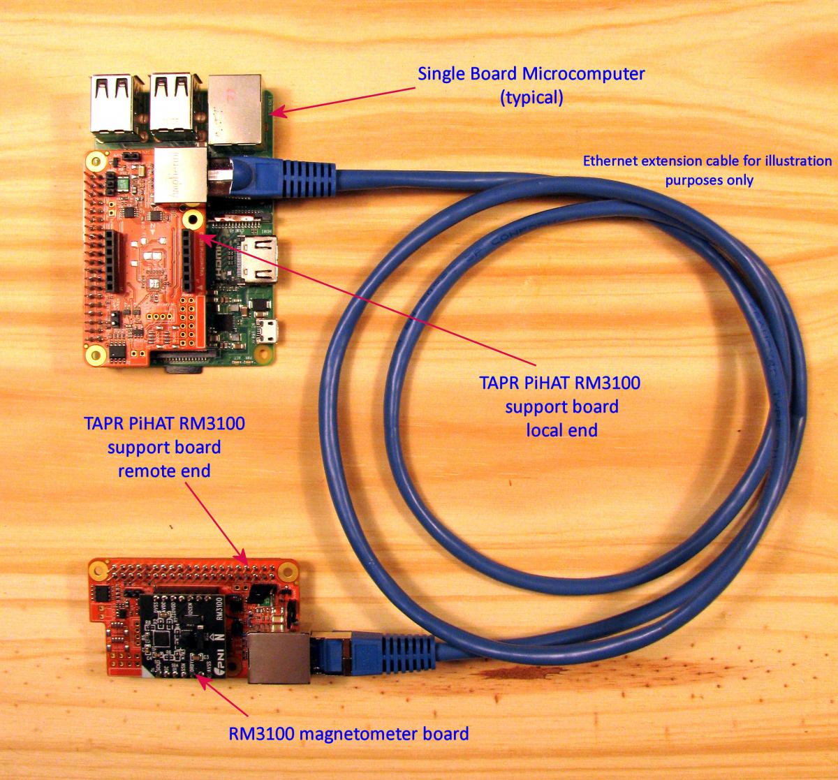
Figure 1. A RM3100 MI magnetometer system (TAPR PiHAT version).
Magnetic Sensor Packaging
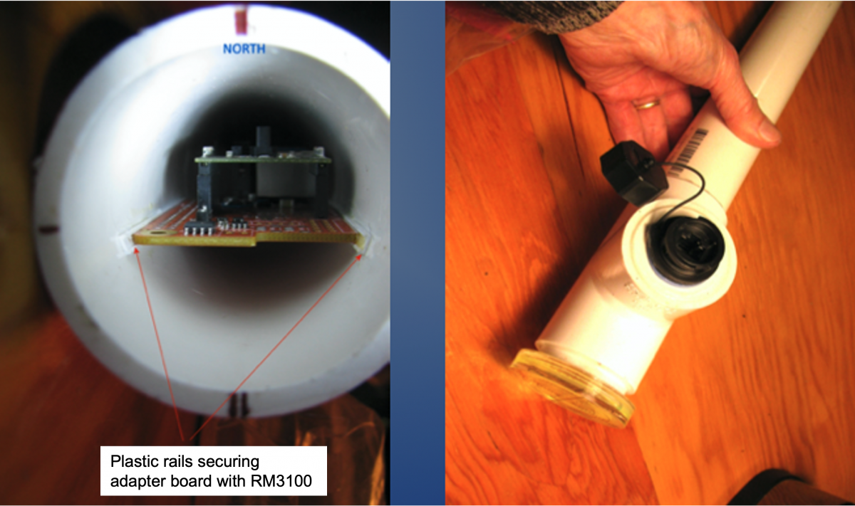
The sensor board (Item #3: remote magnetometer support board extender) is housed in a PVC pipe structure as shown in Figure 2 for weather protection. It can be positioned vertically under the ground so that the sensor, located on the bottom of the pipe, is well below the ground surface level, providing stable temperature (Figure 3). Field installation is shown in Figure 4. Its construction is detailed in a separate document (RM3100 magnetometer assembly in PVC pipe-1.pdf).
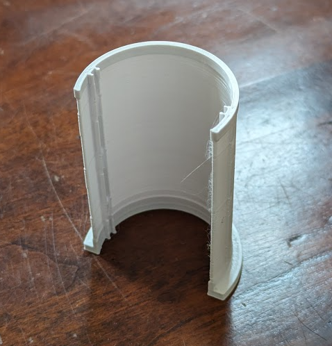
Note1 (April, 2026): A 3D-printed solution for mounting the sensor board in a 2 inch SCH40 plastic pipe now exists. See images here and the STL file for 3D printing here (right click to download). (Thanks to Majid Mokhtari, University of Scranton, for this design.)
Note 2 (April, 2026): A 3D-printed solution for mounting the sensor board in a 1.5 inch SCH40 plastic pipe now exists. See image here. The SCAD file is here and the STL file for 3D printing here (right click to download). (Thanks to Philip Gladstone, N1DQ, for this design.)
Installation and Alignment
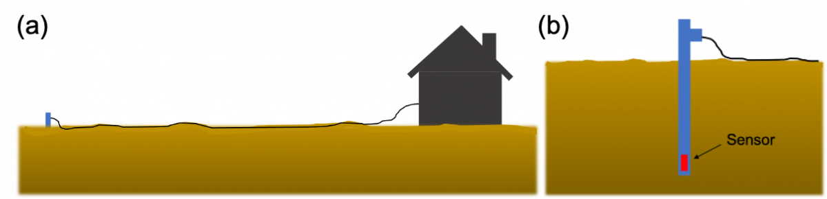
The PVC sensor housing is installed outside of the building where the host computer is located (Figure 3(a)). It is recommended that the sensor is placed at a sufficient distance to avoid any possible EMI source (e.g., the building). A minimum recommended cable length is 100 ft. In an area where EM noise is a concern, use a longer cable (depending on the nature of the noise source). CAT5E and CAT6A can support up to 400 ft and 500 ft, respectively. The cable should be rated for direct burial. The PVC sensor housing is positioned vertically, leaving only the upper part of it (approximately 10 inches) above the ground surface as shown in Figure 3(b) and Figure 4. This provides temperature stability.
The sensor should be oriented in compliance with the widely accepted geomagnetic coordinate system, “HEZ”, in which H points toward the local geomagnetic north in the horizontal plane (perpendicular to the line pointing toward the center of the earth defined as Z). E completes the orthogonal system, pointing toward the geomagnetic east. Thus, Z = H x E in a vector form. Simply, H is defined as a direction which a compass needle would point toward. Figure 4 shows the definition of the coordinate system and the sensor installation conforming to this. It should be noted that the sensor's original XYZ coordinates do not match the HEZ coordinates because of how it is oriented in the pipe (the sensor was designed for use in the horizontal plane, but we are installing it in the vertical plane). Thus, a reallocation of coordinates is required in the post-processing data processing algorithm. That is, H = -Z, E = Y and Z = X where X, Y and Z are the original tri-axial components of the sensor output while H, E and Z are the local geomagnetic components that will be used for scientific use.
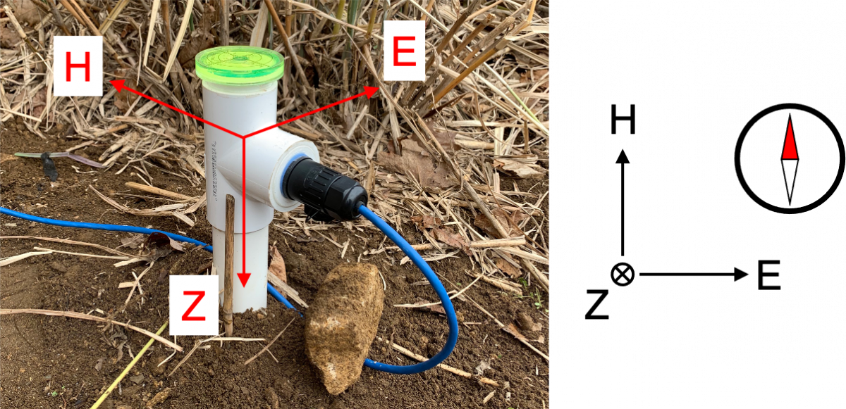
Figure 4. RM3100 sensor PVC pipe packaging installed on the ground.
- Bury the PVC housing in a vertical position, leaving only the upper part of it (approximately 10 inches) above the ground surface. Make sure the pipe is well leveled (using the bubble level on top of it) so it is “vertical” (i.e., aligned with the line toward the center of the earth) and can be rotated freely in the horizontal direction.
- Find the direction of an approximate geomagnetic north, for example, using a compass and orient the pipe so the vertical line marked on the housing (see Figure 2) points toward the geomagnetic north.
- Turn on the magnetometer data acquisition system and run the acquisition software (refer to the operation software document provided separately).
- While one person stays with the sensor outside, the other person monitors data output from the acquisition system.
- While monitoring the horizontal components of the data (H and E), rotate the pipe until the maximum positive value of H and near-zero value of E are obtained.
- Repeat the procedure #5 until reliable horizontal values (H and E) are obtained. This step is particularly important during a geomagnetically disturbed time. Note that for geospace studies, magnetic field “variations” or “pulsations” are more important than absolute values of the fields. Thus, an extreme precision of sensor orientation is not required (as is done for magnetic field observations for geological or geophysical studies).
Initial Data Verification
A “quick and dirty” way to ensure the operation and data quality of the installed magnetometer is to compare the data with the predicted values from a model called International Geomagnetic Reference Field (IGRF), an approximate model field at a particular location. The IGRF can be obtained on a user-friendly website run by Kyoto University. The only information necessary for the model field is the geographic coordinates and altitudes of the magnetometer location and the year of interest. Figure 5 presents a snapshot of the website for model magnetic field at Hope, New Jersey (41N, 75W). The altitude does not need to be very accurate (0 m was entered in this case). It is important to note that the “northward (X)” and “eastward (Y)” in the IGRF are different from our “H” and “E” as the IGRF reports “geographic” north and east whereas our system reports “geomagnetic” north and east. Thus these two values should NOT be compared directly. They are related by X = H * cos (D) where D is declination, the angle on the horizontal plane between magnetic north and true north. Nevertheless, the total “horizontal” field should be close to each other: that is, horizontal = sqrt(X2+Y2) = sqrt(H2+E2). Likewise, the “downward (Z)” should also be close. In addition, the total field can be compared to see if they are similar, as defined as sqrt(X2+Y2+Z2) = sqrt(H2+E2+Z2). Note this is labeled as “F” (total intensity) on the IGRF website. The IGRF values are only from a model and thus it is natural that there are some discrepancies between the actual measurements and the IGRF values. This can be more extreme at high latitudes and/or during geomagnetically disturbed times.
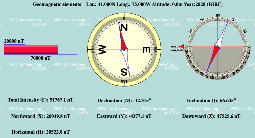
Figure 5. An example of IGRF model magnetic field at Hope, New Jersey (41N, 75W, 0-m altitude) in 2020.
References
Regoli, L. H., Moldwin, M. B., Pellioni, M., Bronner, B., Hite, K., Sheinker, A., and Ponder, B. M.: Investigation of a low-cost magneto-inductive magnetometer for space science applications, Geosci. Instrum. Method. Data Syst., 7, 129–142, https://doi.org/10.5194/gi-7-129-2018, 2018.
The HamSCI Magnetometer Documentation is © Author(s) 2023. This work is distributed under the Creative Commons Attribution 4.0 License.